Examples
#include <numerics.hpp>

int main() {
    const double sigma = 10.0, rho = 28.0, beta = 8.0 / 3.0;

    auto lorenz = [&](double, const num::Vector& s, num::Vector& ds) {
        ds[0] = sigma * (s[1] - s[0]);
        ds[1] = s[0] * (rho - s[2]) - s[1];
        ds[2] = s[0] * s[1] - beta * s[2];
    };

    num::Series xz;
    auto observer = [&](double, const num::Vector& y) {
        xz.store(y[0], y[2]);
    };

    num::solve(
        num::ODEProblem{lorenz, {1.0, 0.0, 0.0}, 0.0, 50.0},
        num::RK45{.rtol = 1e-8, .atol = 1e-10, .max_steps = 2000000},
        observer);

    num::plt::plot(xz);
    num::plt::title("Lorenz attractor (sigma=10, rho=28, beta=8/3)");
    num::plt::xlabel("x");
    num::plt::ylabel("z");
    num::plt::savefig("lorenz.png");
}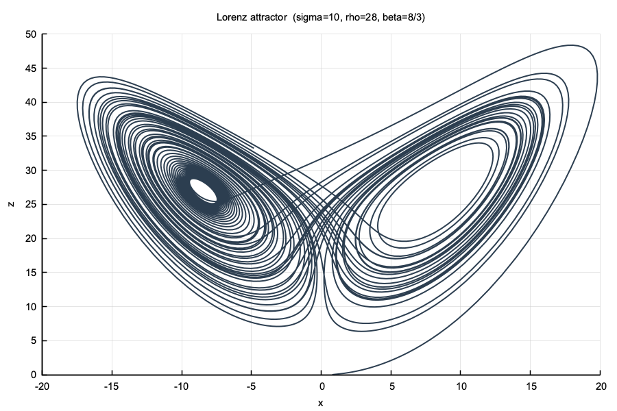
Lorenz attractor — adaptive RK45 via
num::solve + num::RK45#include <numerics.hpp>
#include <cmath>
#include <numbers>
int main() {
constexpr int N = 1024;
constexpr double fs = 1000.0;
constexpr double pi = std::numbers::pi;
num::Vector x(N);
for (int i = 0; i < N; ++i)
x[i] = std::sin(2.0 * pi * 50.0 * i / fs)
+ 0.5 * std::sin(2.0 * pi * 120.0 * i / fs);
num::CVector X(N / 2 + 1);
num::spectral::rfft(x, X);
num::Series signal, spectrum;
for (int i = 0; i < 100; ++i)
signal.store(i / fs * 1000.0, x[i]);
for (num::idx k = 0; k < X.size(); ++k)
spectrum.store(k * fs / N, std::abs(X[k]));
num::plt::subplot(2, 1);
num::plt::plot(signal);
num::plt::title("Signal: 50 Hz + 0.5 * 120 Hz");
num::plt::xlabel("time (ms)"); num::plt::ylabel("amplitude");
num::plt::next();
num::plt::plot(spectrum);
num::plt::title("FFT power spectrum");
num::plt::xlabel("frequency (Hz)"); num::plt::ylabel("|X[k]|");
num::plt::savefig("fft_demo.png");
}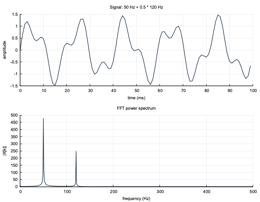
FFT power spectrum —
num::spectral::rfft; peaks at 50 Hz and 120 Hz#include <numerics.hpp>
#include <algorithm>
#include <cmath>
#include <numeric>
#include <random>
#include <vector>
int main() {
constexpr int N = 64;
constexpr int NN = N * N;
num::PBCLattice2D nbr(N);
std::vector<double> spins(NN);
std::mt19937 rng(42);
num::Series curve;
for (double T = 0.5; T <= 4.01; T += 0.1) {
std::fill(spins.begin(), spins.end(), 1.0);
double beta = 1.0 / T;
auto accept = [&](int i) {
double ns = spins[nbr.up[i]] + spins[nbr.dn[i]]
+ spins[nbr.lt[i]] + spins[nbr.rt[i]];
return num::markov::boltzmann_accept(2.0*spins[i]*ns, beta);
};
auto flip = [&](int i) { spins[i] = -spins[i]; };
auto measure = [&]() {
return std::abs(std::accumulate(spins.begin(), spins.end(), 0.0) / NN);
};
double m = num::solve(
num::MCMCProblem{accept, flip, NN},
num::Metropolis{.equilibration = 2000, .measurements = 500},
measure, rng);
curve.store(T, m);
}
num::plt::plot(curve);
num::plt::xlabel("T"); num::plt::ylabel("|<m>|");
num::plt::savefig("ising_demo.png");
}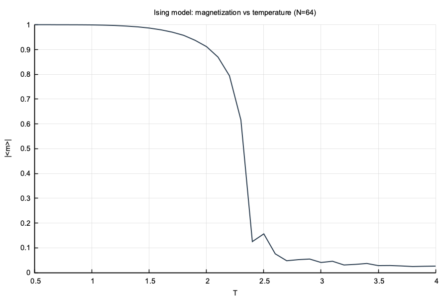
Ising phase transition —
num::solve + num::Metropolis; |m| drops at Tc ≈ 2.27#include <numerics.hpp>
#include <string>
int main() {
constexpr int N = 64;
constexpr double kappa = 1.0, sigma = 0.06, t_end = 0.012;
constexpr double h = 1.0 / (N + 1);
constexpr double dt = 4.0 * h * h;
const int nstep = static_cast<int>(t_end / dt) + 1;
const double coeff = kappa * dt / (h * h);
num::Grid2D grid{N, h};
num::SparseMatrix A = num::pde::backward_euler_matrix(grid, coeff);
num::operators::SparseOp Aop(A);
num::LinearSolver solver = [&](const num::Vector& rhs, num::Vector& x) {
return num::cg(Aop, rhs, x, 1e-8);
};
num::ScalarField2D u0(grid, [=](double x, double y) {
return num::gaussian2d(x, y, 0.5, 0.5, sigma);
});
num::ScalarField2D u = u0;
num::solve(u, num::BackwardEuler{.solver = solver, .dt = dt, .nstep = nstep});
num::plt::subplot(1, 2);
num::plt::heatmap(u0); num::plt::title("t = 0");
num::plt::next();
num::plt::heatmap(u); num::plt::title("t = " + std::to_string(t_end));
num::plt::savefig("heat_demo.png");
}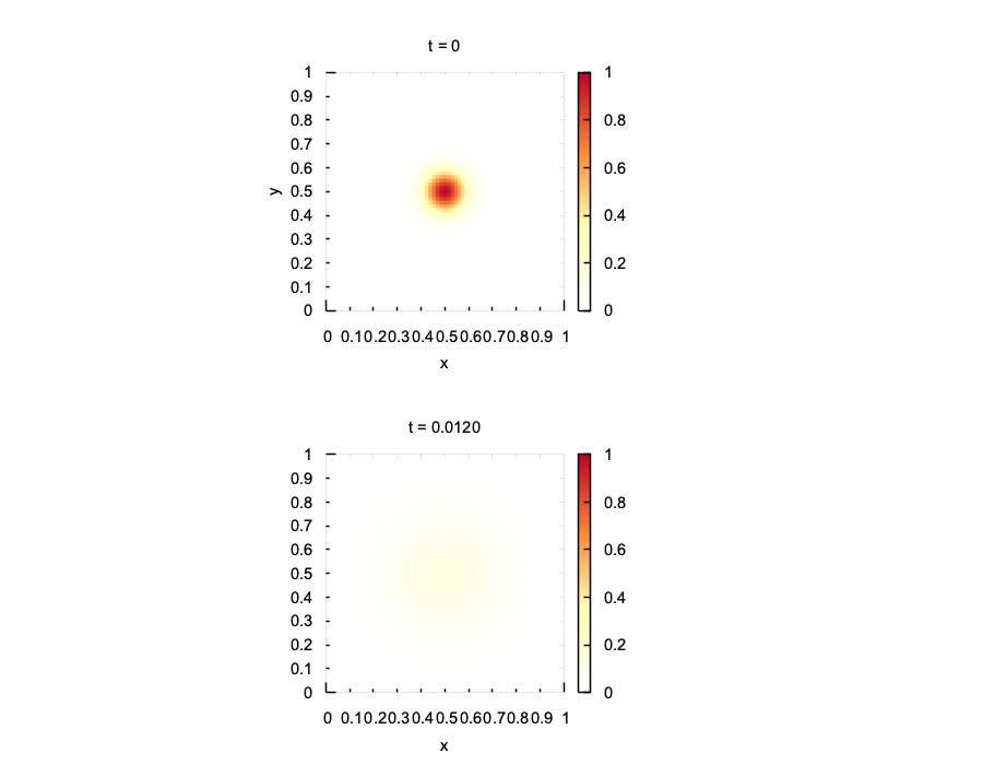
2D heat equation — backward Euler with sparse CG operator;
num::solve + num::BackwardEuler